Attention mechanism for non-Euclidean spaces
Looking at the geometric assumptions behind attention.

Main takeaway: When attention is used on data that has a geometric interpretation— like warped images, spheres, 360° video—the ideal operation is computing a continuous attention integral over the entire domain. In practice, this is not possible. We therefore compute a discrete approximation, i.e., discrete attention between different tokens. To do this correctly, we should take into account not only how tokens relate to each other but also how much area or volume each token represents. The practical solution is simple: add correct weights (the area of the patch) to make the attention geometry-aware.
*Note for readers: Substack still has issues rendering LaTex. In case you do not see rendered equations, I’ve found reloading the substack directly in the browser helps.
1. Attention for non-Euclidean domains: why should we care?
The reason we should care about attention for non-Euclidean spaces rests on three premises:
Premise 1: Many important tasks have intrinsic structure that is not “flat”. This includes graphs (e.g. modeling molecules), spheres (e.g. modeling weather) or other curved domains (e.g. 360° videos).
Premise 2: Standard attention in Transformers compares items using the dot product in a flat vector space and uses positional hacks to inject structure.
Premise 3: In domains where intrinsic structure matters, positional hacks become either suboptimal or insufficient and we need to make the attention mechanism itself aware of the geometry.
If you accept these premises, you should agree that understanding how to use attention in non-Euclidean domains can improve the performance on such structures. Given that there are many unsolved tasks in these domains, and that the attention mechanism has been the primary algorithmic driver behind the success of many deep learning methods, it warrants understanding how to generalize the attention mechanism to these curved domains.
This blog post is inspired by the great work by a team from NVIDIA that published a way to generalize attention on the sphere (and released CUDA kernels for neighborhood attention computation). Check the paper out!
In what follows, I’ll assume the example of modeling the sphere to motivate how attention can be generalized to non-Euclidean domains.
2. Recap of attention
Setup. We have tokens \(x_1, \ldots, x_n \in \mathbb{R}^{d_{\text{model}}}\). Depending on the problem, our tokens might represent different things. In language modeling, each token is a sub-word unit that is represented by a long learned vector; in weather modeling, the token represents an area on the sphere with each channel being, for instance, a climatological measurement; in computer vision, each token represents a group of pixels and their learned embeddings.
For attention, we require learning three linear maps from the token to three other vectors. These three maps are learned and shared across all tokens:
The query: \(q(\cdot): \mathbb{R}^{d_{\text{model}}} \to \mathbb{R}^{d_{k}}\)
The key: \(k(\cdot): \mathbb{R}^{d_{\text{model}}} \to \mathbb{R}^{d_{k}}\)
The value: \(v(\cdot): \mathbb{R}^{d_{\text{model}}} \to \mathbb{R}^{d_{v}}\)
Therefore, each token now has three vectors associated with it. Suppose you’re at token \(x\) and you’re interested in computing the attention scores between \(x\) and all other tokens.
Standard attention can be separated out into three conceptual steps. First, computing the score between the query of \(x\) and the key of another token. Second, computing the softmax weights between the query of \(x\) and all other keys. Third, take a weighted sum of the values using the softmax weights. In more detail:
Step 1. Compute the dot product between the query of \(x\) and the key of another token.
For our token \(x\) and a single other token \(x_j\), we obtain the score by computing their dot product and dividing by the square root of query/key dimensions to keep the variance the same:
\[s_j = \frac{q(x) \cdot k(x_j)}{\sqrt{d_k}}\].
Step 2. Computing the weights between the query of \(x\) and all other keys.
We now need to convert our score into a probability distribution over the keys. This answers the question: “given this query, how much weight should I place on each key?” So, the score for key \(j\) becomes:
\[\alpha_j = \frac{\exp(s_j)}{\sum_{i=1}^n \exp(s_i)}.\]
Step 3. Take a weighted sum of the values using the softmax weights. The query computes a weighted sum of the values:
\[\text{Attn}(x) = \sum_{j=1}^n \alpha_j(x)\, v(x_j).\]
3. Attention assumes each token covers the same area
Vanilla attention uses a dot-product similarity in embedding space and implicitly assumes each token covers the same area/volume. If we are operating on a continuous space where tokens correspond to regions with area, the average is a modeling approximation to an integral (with respect to the domain’s measure). To do it perfectly, we would need to integrate over the area. However, this is almost always impossible and we therefore use a weighted sum, with a particular weight per token.
So, the standard attention formula relies on the scores \(\alpha_j\) and \(v(\cdot)\).
\[\text{Attn}(x) \approx \sum_{j=1}^n \alpha_j(x)\, v(x_j)\].
This becomes an approximation only if we are indeed approximating a continuous domain. We can explicitly include the size of the region of this area as follows:
\[\text{Attn}(x) \approx \sum_{j=1}^n \alpha_j(x)\, v(x_j)\, \underbrace{(\text{area of cell } j)}_{\text{Include this.}}\]
When tokens correspond to regions of a continuous domain, vanilla attention leaves out the “area of a cell” factor. This is alright in case the areas are the same. When areas differ—e.g. a sphere—we should include a weighting of that area. Here, \(\alpha_j\) represents similarity from the softmax and \(\omega_j\) accounts for the cell area. At this stage, we still have to renormalize attention (we have added area weights but have not divided by the normalization constant that makes the weights sum to 1).
To understand how to do this, let’s look at the sphere as an example.
4. Size of an area and the sphere
On a flat plane, dividing the space into equal squares means every cell has the same area. But the sphere is curved. Therefore, equal steps in latitude and longitude do not correspond to equal surface area. We typically divide the sphere into grids which are represented by intersections of latitude-longitude.
Therefore, for our attention formula, we need to account for these differences in sizes. We can now ask: how should we weight each area according to its size?
The answer lies in computing the actual area of each grid cell. On a unit sphere, a small patch of area dA can be expressed as dA = (height) (width), where we parameterize position using two angles:
\(\theta\) to denote how far down the North Pole we are (0 at the North Pole, \(\pi\) at the South Pole). This convention is referred to as colatitude.
\(\phi\) to denote how far around the sphere—longitude.
The area for a tiny area on a sphere is then
\[dA = \underbrace{d\theta}_{\text{height}}\underbrace{\sin\theta d\phi}_{\text{width}}\].
Explaining the height. On a unit sphere, the colatitude angle \(\theta\) measures your angular position from the North Pole. For each meridian line (i.e. the longitude line), the radius \(\rho\) (depicted in green in the figure below) is 1. If we move along the same meridian line further away from the North Pole, we will have moved along the arc by a distance of radius \(\times d\theta\) which is just \(d\theta\)—obtained by applying the fundamental rule: arc-length = radius \(\times\) angle. Intuitively: if you have not moved, then your arc length is zero. If you’ve moved 90 degrees (\( \frac{\pi}{2}\) units), your arc length is \( \frac{\pi}{2} \approx 1.57\) units.
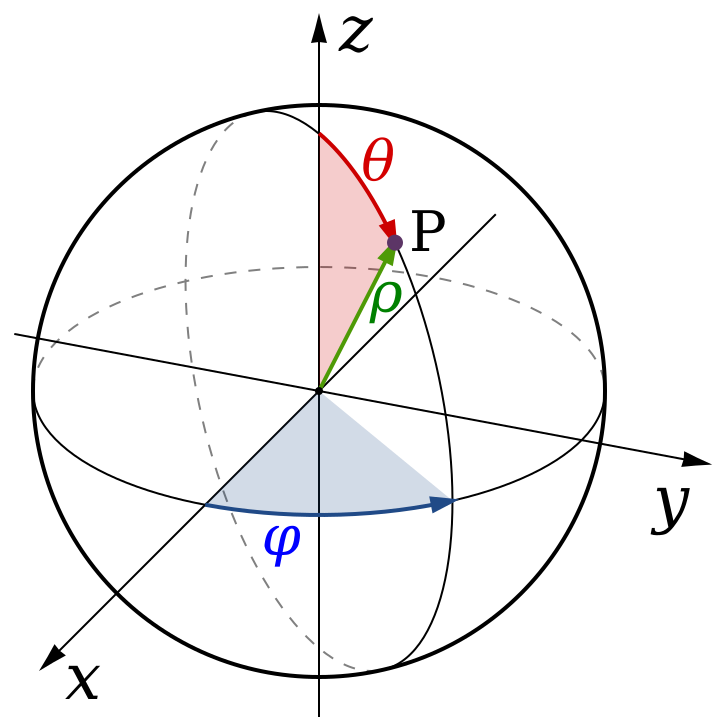
Explaining the width. At colatitude \(\theta\), you’re standing on a small circle (a latitude line). The radius of this circle is \(\sin(\theta)\). When you move through a small longitude angle \(d\phi\), you trace an arc along this smaller circle. Therefore, the width will be \(\sin(\theta) \times d\phi\).
Combining the width and height together, we obtain \(dA = \sin\theta d\theta d\phi\).
5. Attention performed on a sphere
We will now use two facts we’ve built up:
Standard attention implicitly assumes equal area/volume represented by each token.
We have computed a way to weigh the area of a specific token on a sphere.
Now, let’s fix vanilla attention by incorporating the weighting scheme we have introduced. Recall the standard vanilla attention formula:
\[\text{Attn}(x) = \sum_{j=1}^n \alpha_j(x)\, v(x_j).\]
Then a faithful spherical average must be weighted by the area. If we introduce the area as \(\omega\), then our attention becomes:
\[\text{Attn}(x) \approx \sum_{j=1}^n \alpha_j(x)\, v(x_j) \omega_j.\]
That is, in effect, all there is to it.
We can still do a bit more to be very precise. Notice that both \(\alpha\) and \(\omega\) are encoding some sort of weighting: \(\alpha\) is encoding post-softmax weights and \(\omega\) is encoding quadrature weights. We can combine them such that there is a single set of probabilities that reflect, simultaneously, the importance and area of each cell.
Recall the attention weights are \[\alpha_j = \frac{\exp(s_j)}{\sum_{i=1}^n \exp(s_i)}.\] We can re-define the weights to mean both similarity and area, and then normalize by softmax. Two changes must then be made: (1) on the numerator, we should multiply by the weight of the cell with which we are computing attention to; (2) on the denominator, we need to ensure the weights still sum to 1 for it to form a valid probability distribution. Therefore, our new weights are:
\[\tilde{\alpha}_j = \frac{\exp(s_j)\omega_j}{\sum_i\exp(s_i)\omega_i}\]
There’s one final trick we can do to make the calculations easier. Recall the property that exponential terms can be separated out within an exponent:
Another way to look at this is that if you have an exponent multiplied by a term (like a weight), this is equivalent to adding the term with a log inside the exponent:
\[\exp(a) \cdot b = \exp(a + \log{b})\].
Therefore, instead of multiplying the exponentiated scores by the area weight, we can move the area weight into the exponentiation term. As we have just seen, this can be done by converting the multiplication of the area weights into an addition of a logarithmic term:
\[\tilde{\alpha}_j = \frac{\exp(s_j + \log{\omega_j})}{\sum_i\exp(s_i + \log{\omega_i})}\]
(we typically add a small number to the weight before the log to avoid \(\omega_j\) being exactly zero, since \(\log(0)\) is undefined).
And recall that we’ve already found the weights of the area: they are proportional to the change in the area in the grid, \(\omega_j \propto \sin(\theta_j)\). We only need the weights to be proportional to \(\sin(\theta_j)\) because any uniform constant factor, such as the common factors \(d\theta\) and \(d\phi\), multiplies every cell equally and cancels out when you normalize the weights. In other words, only relative variation with latitude matters; and this is exactly what \(\sin(\theta_j)\) represents.
6. Why do we treat tokens in language models as if they come from a Euclidean space?
We do not apply any sort of weighting schemes or area representation to token embeddings in language models. Why?
Vector embeddings for words are Euclidean by construction. We map each token into a vector in some high-dimensional space and perform operations like dot products assuming standard linear geometry. This works because embeddings are trained to approximately follow this Euclidean geometry.
That is not to say that this is “optimal”. It could be that treating vectors in non-Euclidean space would be a much better choice, as discussed in various works.